<?xml version="1.0" encoding="utf-8"?><feed xmlns="http://www.w3.org/2005/Atom" ><generator uri="https://jekyllrb.com/" version="3.10.0">Jekyll</generator><link href="https://rubaduckduck.github.io/feed.xml" rel="self" type="application/atom+xml" /><link href="https://rubaduckduck.github.io/" rel="alternate" type="text/html" /><updated>2025-05-14T16:25:51+00:00</updated><id>https://rubaduckduck.github.io/feed.xml</id><title type="html">Blog</title><subtitle>Description.</subtitle><author><name>Jung Hoe, Hur</name></author><entry><title type="html">Beyond Hierarchy: Rethinking Visual Processing in the Brain</title><link href="https://rubaduckduck.github.io/2025/05/14/about_vision.html" rel="alternate" type="text/html" title="Beyond Hierarchy: Rethinking Visual Processing in the Brain" /><published>2025-05-14T00:00:00+00:00</published><updated>2025-05-14T00:00:00+00:00</updated><id>https://rubaduckduck.github.io/2025/05/14/about_vision</id><content type="html" xml:base="https://rubaduckduck.github.io/2025/05/14/about_vision.html"><![CDATA[<p>For decades, our understanding of visual processing in the brain has been dominated by hierarchical models. Much like modern convolutional neural networks (CNNs), we’ve envisioned a system where simple features are detected first, then progressively combined into more complex representations as information travels through successive neural layers. But what if this fundamental assumption is flawed?</p>

<h2 id="the-limits-of-hierarchical-processing">The Limits of Hierarchical Processing</h2>

<p>The conventional model suggests that our visual system is structured like a deep neural network—with early layers detecting edges and colors, middle layers identifying shapes and textures, and deeper layers recognizing objects and scenes. This neat, linear progression feels intuitive, but it fails to explain several remarkable human visual capabilities.</p>

<p>Consider a thought experiment: imagine the letter “A” composed of tiny letter “A”s, which themselves are made of even smaller “A”s, continuing infinitely. A hierarchical system would eventually hit a limit—running out of processing layers to handle deeper levels of recursion. Yet humans effortlessly perceive the pattern at multiple scales simultaneously. We recognize both the large “A” and, upon closer inspection, the smaller “A”s that compose it, regardless of how many levels deep the pattern goes.</p>

<p>This recursive pattern recognition isn’t limited to letters. We see it in our ability to process nested visual structures in nature, art, and design. Whether it’s recognizing a forest, then the trees that comprise it, then the branches, leaves, and cellular structures—our visual system seems to apply the same recognition mechanisms recursively at different scales.</p>

<h2 id="the-recursive-alternative">The Recursive Alternative</h2>

<p>What if, instead of a hardwired hierarchy, our visual system employs a more flexible, recursive approach? Drawing inspiration from computer science, we might compare the brain to a CPU handling recursive functions. Despite having limited physical depth, a single processor can navigate arbitrarily deep recursive structures using a stack mechanism—pushing and popping information as needed.</p>

<p>Similarly, the brain might use a core set of neural operations that can be dynamically applied at different levels of abstraction. Rather than having dedicated neural circuits for each level of visual complexity, the same neural machinery might process different levels of detail through recurrent connections and attentional mechanisms.</p>

<p>This perspective aligns with several emerging theories in neuroscience:</p>

<ol>
  <li>
    <p><strong>Predictive coding models</strong> suggest the brain uses a common operation—minimizing prediction error—throughout the visual system, rather than fundamentally different operations at each level.</p>
  </li>
  <li>
    <p><strong>Recurrent processing theories</strong> emphasize that visual processing isn’t just a feedforward cascade but involves extensive feedback and lateral connections, allowing the same neural populations to participate in different levels of processing.</p>
  </li>
  <li>
    <p><strong>Global workspace theories</strong> propose that conscious perception involves broadcasting information to a shared neural workspace where the same mechanisms can operate on different levels of abstraction.</p>
  </li>
</ol>

<h2 id="implications-for-artificial-intelligence">Implications for Artificial Intelligence</h2>

<p>If this recursive model better reflects human vision, it suggests we might need to rethink the purely hierarchical architectures that dominate computer vision today. While modern CNNs have achieved remarkable results, they still struggle with the kind of flexible, scale-invariant processing that humans perform effortlessly.</p>

<p>Systems incorporating more recurrent processing, attention mechanisms, and working memory-like components might better capture the recursive nature of visual intelligence. Rather than adding more layers, we might need architectures that can dynamically apply the same operations at different scales and levels of abstraction.</p>

<h2 id="a-new-perspective">A New Perspective</h2>

<p>The recursive view of visual processing invites us to question a fundamental assumption in neuroscience and AI. Perhaps the brain’s remarkable efficiency stems not from having specialized circuits for every level of visual complexity, but from its ability to apply the same fundamental operations recursively across different scales and contexts.</p>

<p>This perspective might help explain why humans show remarkable invariance to scale, position, and viewpoint that still challenges deep learning systems. We’re not just processing images through a fixed hierarchy—we’re dynamically engaging with visual information at multiple levels of abstraction using the same core neural mechanisms.</p>

<p>As we continue to unravel the mysteries of visual perception, perhaps it’s time to look beyond the comforting ladder of hierarchy and embrace the more versatile spiral of recursion.</p>]]></content><author><name>Jung Hoe, Hur</name></author><category term="Other" /><summary type="html"><![CDATA[For decades, our understanding of visual processing in the brain has been dominated by hierarchical models. Much like modern convolutional neural networks (CNNs), we’ve envisioned a system where simple features are detected first, then progressively combined into more complex representations as information travels through successive neural layers. But what if this fundamental assumption is flawed? The Limits of Hierarchical Processing The conventional model suggests that our visual system is structured like a deep neural network—with early layers detecting edges and colors, middle layers identifying shapes and textures, and deeper layers recognizing objects and scenes. This neat, linear progression feels intuitive, but it fails to explain several remarkable human visual capabilities. Consider a thought experiment: imagine the letter “A” composed of tiny letter “A”s, which themselves are made of even smaller “A”s, continuing infinitely. A hierarchical system would eventually hit a limit—running out of processing layers to handle deeper levels of recursion. Yet humans effortlessly perceive the pattern at multiple scales simultaneously. We recognize both the large “A” and, upon closer inspection, the smaller “A”s that compose it, regardless of how many levels deep the pattern goes. This recursive pattern recognition isn’t limited to letters. We see it in our ability to process nested visual structures in nature, art, and design. Whether it’s recognizing a forest, then the trees that comprise it, then the branches, leaves, and cellular structures—our visual system seems to apply the same recognition mechanisms recursively at different scales. The Recursive Alternative What if, instead of a hardwired hierarchy, our visual system employs a more flexible, recursive approach? Drawing inspiration from computer science, we might compare the brain to a CPU handling recursive functions. Despite having limited physical depth, a single processor can navigate arbitrarily deep recursive structures using a stack mechanism—pushing and popping information as needed. Similarly, the brain might use a core set of neural operations that can be dynamically applied at different levels of abstraction. Rather than having dedicated neural circuits for each level of visual complexity, the same neural machinery might process different levels of detail through recurrent connections and attentional mechanisms. This perspective aligns with several emerging theories in neuroscience: Predictive coding models suggest the brain uses a common operation—minimizing prediction error—throughout the visual system, rather than fundamentally different operations at each level. Recurrent processing theories emphasize that visual processing isn’t just a feedforward cascade but involves extensive feedback and lateral connections, allowing the same neural populations to participate in different levels of processing. Global workspace theories propose that conscious perception involves broadcasting information to a shared neural workspace where the same mechanisms can operate on different levels of abstraction. Implications for Artificial Intelligence If this recursive model better reflects human vision, it suggests we might need to rethink the purely hierarchical architectures that dominate computer vision today. While modern CNNs have achieved remarkable results, they still struggle with the kind of flexible, scale-invariant processing that humans perform effortlessly. Systems incorporating more recurrent processing, attention mechanisms, and working memory-like components might better capture the recursive nature of visual intelligence. Rather than adding more layers, we might need architectures that can dynamically apply the same operations at different scales and levels of abstraction. A New Perspective The recursive view of visual processing invites us to question a fundamental assumption in neuroscience and AI. Perhaps the brain’s remarkable efficiency stems not from having specialized circuits for every level of visual complexity, but from its ability to apply the same fundamental operations recursively across different scales and contexts. This perspective might help explain why humans show remarkable invariance to scale, position, and viewpoint that still challenges deep learning systems. We’re not just processing images through a fixed hierarchy—we’re dynamically engaging with visual information at multiple levels of abstraction using the same core neural mechanisms. As we continue to unravel the mysteries of visual perception, perhaps it’s time to look beyond the comforting ladder of hierarchy and embrace the more versatile spiral of recursion.]]></summary></entry><entry><title type="html">The Unified Field of Sensation: How We Compare Experiences Across Space</title><link href="https://rubaduckduck.github.io/2025/05/14/unified_field_of_sensation.html" rel="alternate" type="text/html" title="The Unified Field of Sensation: How We Compare Experiences Across Space" /><published>2025-05-14T00:00:00+00:00</published><updated>2025-05-14T00:00:00+00:00</updated><id>https://rubaduckduck.github.io/2025/05/14/unified_field_of_sensation</id><content type="html" xml:base="https://rubaduckduck.github.io/2025/05/14/unified_field_of_sensation.html"><![CDATA[<p>Light reaches the retina, becomes neural signals, and then we see the world. This transformation—from photons to conscious experience—happens so seamlessly that we rarely pause to consider its profound implications.</p>

<h2 id="the-mystery-of-sensory-comparison">The Mystery of Sensory Comparison</h2>

<p>One of the most remarkable yet overlooked aspects of perception is our ability to compare sensations across different regions of our sensory fields. Consider color: when you look at a blue sky, the “blueness” you experience in the upper left corner of your visual field is immediately comparable to the “blueness” in the upper right corner. Despite these sensations originating from entirely different photoreceptors in physically separate parts of your retina, you effortlessly recognize them as the same color.</p>

<p>This capability extends beyond vision. With touch, we can feel similar sensations on widely separated parts of our body and recognize their similarity. A gentle pressure applied to your left hand feels qualitatively similar to the same pressure applied to your right foot, despite these sensations originating from completely different nerve endings separated by considerable physical distance.</p>

<p>The same principle applies to temperature, itch, pain, and other bodily sensations. We can compare the intensity of an itch on our back with one on our arm, or recognize that the temperature of water on our left hand matches that on our right.</p>

<h2 id="beyond-connectivity">Beyond Connectivity</h2>

<p>What makes this ability so remarkable is that there’s no direct physical connection between the receptors involved. The photoreceptors in one part of your retina don’t connect directly to those in another part. The touch receptors in your hand have no direct neural pathway to those in your foot.</p>

<p>Yet somehow, our brain constructs a unified sensory field where these disparate signals can be compared, contrasted, and integrated into a coherent experience. The signals from physically distant receptors must be transformed into a common “neural language” or representational space where comparison becomes possible.</p>

<p>This transformation transcends the physical arrangement of our sensory apparatus. It suggests that our brain doesn’t just process sensory data—it creates a unified experiential field where sensations acquire qualities that can be compared across space.</p>

<h2 id="implications-for-consciousness-and-artificial-intelligence">Implications for Consciousness and Artificial Intelligence</h2>

<p>This observation has profound implications for our understanding of consciousness and the development of truly feeling artificial systems.</p>

<p>For consciousness, it suggests that creating a unified field of comparable sensations might be one of the fundamental operations that transforms mere signal processing into subjective experience. The ability to compare sensations across space may be integral to what philosophers call “qualia”—the subjective qualities of experience.</p>

<p>For artificial intelligence and robotics, this insight points to a crucial missing piece in our attempts to create machines that can “feel.” A robot with sensors distributed across its body doesn’t just need to register input from these sensors—it needs neural architecture that transforms these spatially distinct signals into a unified representational space where sensations can be compared and integrated.</p>

<p>Current AI systems process inputs from different sensors separately or merge them in simplistic ways. They lack the unified sensory field that allows for the rich, qualitative comparisons that characterize human experience. Even the most advanced deep learning systems don’t create the kind of representational space where a sensation in one part of the system can be qualitatively compared to a sensation in another part.</p>

<h2 id="the-bridge-to-feeling">The Bridge to Feeling</h2>

<p>Understanding how our brain creates this unified field of comparable sensations may be the key to developing artificial systems that truly “feel” rather than merely “sense.” It might be the bridge between data processing and consciousness—the ability to create a unified experiential field from distributed sensory inputs.</p>

<p>This is not merely a technical challenge but a profound philosophical one. It requires us to understand how physical systems like brains transform spatially distinct signals into a unified field of comparable experiences—how the firing of neurons becomes the rich, integrated tapestry of conscious perception.</p>

<p>By exploring this fundamental aspect of perception, we might not only deepen our understanding of human consciousness but also chart a path toward artificial systems that don’t just mimic the outward behaviors of sentient beings but share something of their inner experience as well.</p>

<p>The ability to compare blue in one part of your visual field with blue in another might seem trivial, but it points to one of the deepest mysteries of consciousness—how physically separate neural processes give rise to a unified field of experience where sensations can be compared across space.</p>]]></content><author><name>Jung Hoe, Hur</name></author><category term="Other" /><summary type="html"><![CDATA[Light reaches the retina, becomes neural signals, and then we see the world. This transformation—from photons to conscious experience—happens so seamlessly that we rarely pause to consider its profound implications. The Mystery of Sensory Comparison One of the most remarkable yet overlooked aspects of perception is our ability to compare sensations across different regions of our sensory fields. Consider color: when you look at a blue sky, the “blueness” you experience in the upper left corner of your visual field is immediately comparable to the “blueness” in the upper right corner. Despite these sensations originating from entirely different photoreceptors in physically separate parts of your retina, you effortlessly recognize them as the same color. This capability extends beyond vision. With touch, we can feel similar sensations on widely separated parts of our body and recognize their similarity. A gentle pressure applied to your left hand feels qualitatively similar to the same pressure applied to your right foot, despite these sensations originating from completely different nerve endings separated by considerable physical distance. The same principle applies to temperature, itch, pain, and other bodily sensations. We can compare the intensity of an itch on our back with one on our arm, or recognize that the temperature of water on our left hand matches that on our right. Beyond Connectivity What makes this ability so remarkable is that there’s no direct physical connection between the receptors involved. The photoreceptors in one part of your retina don’t connect directly to those in another part. The touch receptors in your hand have no direct neural pathway to those in your foot. Yet somehow, our brain constructs a unified sensory field where these disparate signals can be compared, contrasted, and integrated into a coherent experience. The signals from physically distant receptors must be transformed into a common “neural language” or representational space where comparison becomes possible. This transformation transcends the physical arrangement of our sensory apparatus. It suggests that our brain doesn’t just process sensory data—it creates a unified experiential field where sensations acquire qualities that can be compared across space. Implications for Consciousness and Artificial Intelligence This observation has profound implications for our understanding of consciousness and the development of truly feeling artificial systems. For consciousness, it suggests that creating a unified field of comparable sensations might be one of the fundamental operations that transforms mere signal processing into subjective experience. The ability to compare sensations across space may be integral to what philosophers call “qualia”—the subjective qualities of experience. For artificial intelligence and robotics, this insight points to a crucial missing piece in our attempts to create machines that can “feel.” A robot with sensors distributed across its body doesn’t just need to register input from these sensors—it needs neural architecture that transforms these spatially distinct signals into a unified representational space where sensations can be compared and integrated. Current AI systems process inputs from different sensors separately or merge them in simplistic ways. They lack the unified sensory field that allows for the rich, qualitative comparisons that characterize human experience. Even the most advanced deep learning systems don’t create the kind of representational space where a sensation in one part of the system can be qualitatively compared to a sensation in another part. The Bridge to Feeling Understanding how our brain creates this unified field of comparable sensations may be the key to developing artificial systems that truly “feel” rather than merely “sense.” It might be the bridge between data processing and consciousness—the ability to create a unified experiential field from distributed sensory inputs. This is not merely a technical challenge but a profound philosophical one. It requires us to understand how physical systems like brains transform spatially distinct signals into a unified field of comparable experiences—how the firing of neurons becomes the rich, integrated tapestry of conscious perception. By exploring this fundamental aspect of perception, we might not only deepen our understanding of human consciousness but also chart a path toward artificial systems that don’t just mimic the outward behaviors of sentient beings but share something of their inner experience as well. The ability to compare blue in one part of your visual field with blue in another might seem trivial, but it points to one of the deepest mysteries of consciousness—how physically separate neural processes give rise to a unified field of experience where sensations can be compared across space.]]></summary></entry><entry><title type="html">SFENO: A Flexible Framework for Modeling Biological Networks</title><link href="https://rubaduckduck.github.io/2025/02/25/sfeno.html" rel="alternate" type="text/html" title="SFENO: A Flexible Framework for Modeling Biological Networks" /><published>2025-02-25T00:00:00+00:00</published><updated>2025-02-25T00:00:00+00:00</updated><id>https://rubaduckduck.github.io/2025/02/25/sfeno</id><content type="html" xml:base="https://rubaduckduck.github.io/2025/02/25/sfeno.html"><![CDATA[<p>github links:   <br />
<a href="https://github.com/sanderlab/CellBox">Cellbox</a>  <br />
<a href="https://github.com/RubADuckDuck/SFENO_temporary">SFENO</a></p>

<h2 id="introduction-to-sfeno">Introduction to SFENO</h2>

<p>SFENO (Structured Framework for Exploring Network ODEs) is a flexible framework designed to model and simulate biological networks using ordinary differential equations (ODEs). It was developed as an improvement over the existing Cellbox model, addressing key limitations in flexibility, hardware compatibility, and experimental design.</p>

<h2 id="key-limitations-of-cellbox">Key Limitations of Cellbox</h2>

<p>The original Cellbox model had several limitations:</p>

<ol>
  <li>
    <p><strong>Tightly Coupled Architecture</strong>: The ODE equations were deeply embedded within the Cellbox model itself, making it difficult to modify or experiment with different mathematical approaches without rewriting the entire class.</p>
  </li>
  <li>
    <p><strong>Limited Learning Methods</strong>: The learning code was designed specifically for the approach described in the paper, lacking flexibility for applying various learning techniques.</p>
  </li>
  <li>
    <p><strong>Hardware Constraints</strong>: Being implemented in TensorFlow, the code was not easily adaptable to different hardware environments without significant modifications.</p>
  </li>
</ol>

<h2 id="sfenos-architectural-improvements">SFENO’s Architectural Improvements</h2>

<p><img src="/assets/images/about_sfeno.png" alt="Structural differences between Cellbox and SFENO" width="100%" /></p>

<p>SFENO addresses these limitations through several key architectural changes:</p>

<h3 id="1-modular-architecture">1. Modular Architecture</h3>

<p><img src="/assets/images/about_sfeno.png" alt="SFENO" width="100%" /></p>

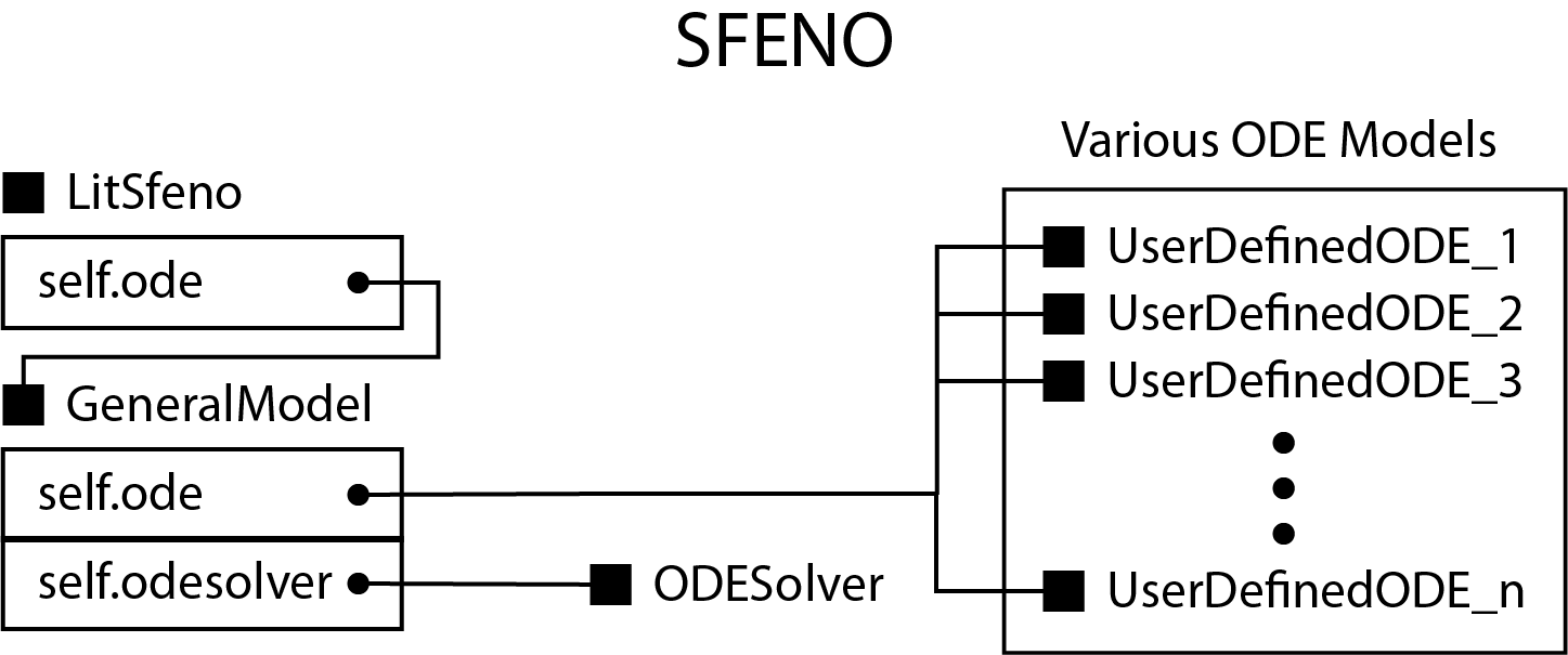
<p>The architecture clearly separates different components:</p>
<ul>
  <li><code>LitSfeno</code>: The top-level wrapper that integrates PyTorch Lightning functionality</li>
  <li><code>GeneralModel</code>: A middle-layer that handles ODE solving and model coordination</li>
  <li>User-defined ODE modules: Customizable components that define how the state changes</li>
</ul>

<p>This separation allows researchers to modify just the ODE equations without changing the rest of the system, significantly enhancing experimental flexibility.</p>

<p>Here’s an example of the <code>LitSfeno</code> class showing how it wraps the model and integrates PyTorch Lightning:</p>

<pre><code class="language-python">class LitSfeno(pl.LightningModule):
    def __init__(self, config, args, ud_class_nm):
        super().__init__()
        
        # Create model using the user-defined ODE class
        self.model = GeneralModel.build_model(config=config,
                                              args=args,
                                              user_defined_dxdt=ud_class_nm,
                                              master=self)
        
        self.lr = 0.001
        self.optimizer = torch.optim.Adam(self.model.parameters(), lr=self.lr)
        
    def forward(self, t, y0, arg_dict):
        return self.model(self, t, y0, arg_dict)
        
    def get_device(self):
        return self.device
        
    def training_step(self, batch, batch_idx):
        inputs, targets = batch
        y0, additional_args = inputs
        
        outputs = self.model(t=0, y0=y0, arg_dict=additional_args)
        loss = self.loss_fn(outputs, targets)
        
        self.log("train_loss", loss, on_step=False, on_epoch=True)
        return loss
</code></pre>

<h3 id="2-pytorch-lightning-integration">2. PyTorch Lightning Integration</h3>

<p>SFENO replaces TensorFlow with PyTorch and introduces PyTorch Lightning, providing:</p>
<ul>
  <li>Hardware agnostic operation across CPUs, GPUs, and TPUs without code changes</li>
  <li>Support for distributed training (DDP - Distributed Data Parallel)</li>
  <li>Built-in callbacks at appropriate points during model training</li>
  <li>Automatic tensor management across devices</li>
</ul>

<p>The following code demonstrates how SFENO leverages PyTorch Lightning for hardware-agnostic training:</p>

<pre><code class="language-python"># Example of setting up training with different hardware configurations
if pargs.ddp:  # Distributed Data Parallel (multi-GPU)
    trainer = Trainer(devices=pargs.num_gpu,
                      accelerator="gpu",
                      max_epochs=config.config['max_epoch'],
                      strategy="ddp_find_unused_parameters_false")
else:  # Single GPU
    trainer = Trainer(devices=pargs.num_gpu,
                      accelerator="gpu",
                      max_epochs=config.config['max_epoch'])

# Train the model with the same code regardless of hardware configuration
trainer.fit(lit_sfeno, datamodule=lit_datamodule)
</code></pre>

<h3 id="3-flexible-masking-system">3. Flexible Masking System</h3>

<p><img src="/assets/images/masking.png" width="100%" /></p>

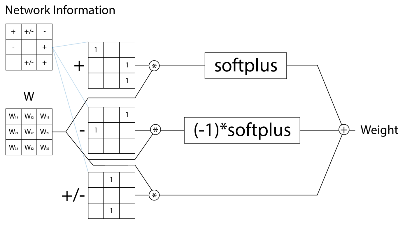
<p>SFENO implements a generalized masking system for network constraints:</p>
<ul>
  <li>Four possible interaction types between nodes: no influence, bidirectional influence, positive-only influence, or negative-only influence</li>
  <li>User-defined network structure information can be directly incorporated</li>
  <li>The <code>StructInfoLayer</code> class manages these constraints through an elegant filtering mechanism</li>
</ul>

<p>Here’s how the masking system is implemented:</p>

<pre><code class="language-python">class StructInfoLayer(nn.Module):
    def __init__(self, config, master):
        super().__init__()
        self.master = [master]
        
        # Initialize adjacency matrix
        if config.adj_mat==1:
            self.adj_mat = np.ones((config.config["n_x"],config.config["n_x"]))
        else:
            self.adj_mat = config.adj_mat
            
        self.node_names = config.node_nm_ls
        self.node_num = len(self.adj_mat)
        
        # Network weight parameters
        self.register_parameter(
            'W', nn.parameter.Parameter(torch.zeros((self.node_num, self.node_num), 
                                                    requires_grad=True))
        )
        
        # Define different parameter transformation functions
        def zero_param(x):
            return x * 0
            
        def R_param(x):
            return x
            
        def R_pos_param(x):
            return F.softplus(x)  # Positive-only influence
            
        def R_ngt_param(x):
            return(-1) * F.softplus(x)  # Negative-only influence
            
        self.adj_val2get_param_func = {
            0: zero_param,      # No influence
            1: R_param,         # Bidirectional influence
            2: R_pos_param,     # Positive-only influence
            3: R_ngt_param      # Negative-only influence
        }

    def load_mask(self):
        # Create masks for each interaction type
        self.mask = torch.zeros(
            (self.node_num, self.node_num),
            requires_grad=False).type_as(next(self.parameters()))
            
        for adj_val, func in self.adj_val2get_param_func.items():
            mask = func(self.W * self.adj_val2mask[adj_val].type_as(next(self.parameters())))
            self.mask = self.mask + mask
</code></pre>

<h3 id="4-easy-experimental-configuration">4. Easy Experimental Configuration</h3>

<p>The framework supports:</p>
<ul>
  <li>Hyperparameter scheduling across training stages</li>
  <li>Custom loss function definitions within user-defined ODE modules</li>
  <li>Automatic network weight saving at specified epochs</li>
  <li>Performance tracking and evaluation</li>
</ul>

<p>Example of implementing a custom ODE function with hyperparameter scheduling:</p>

<pre><code class="language-python">class Example_Cellbox(GeneralODE):
    def __init__(self, config, master):
        super().__init__(config, master)
        
        # Initialize network model with structural information
        self.net_model = StructInfoLayer(config, master=self)
        self.net_model.init_params()
        self.net_model.load_mask()
        
        # Register learnable parameters
        self.register_parameter(
            'epsilon', nn.parameter.Parameter(
                F.softplus(torch.ones((config.config["n_x"]),
                           dtype=torch.float32, requires_grad=True)))
        )
        
        self.register_parameter(
            'alpha', nn.parameter.Parameter(
                F.softplus(torch.ones((config.config["n_x"]),
                           dtype=torch.float32, requires_grad=True)))
        )
        
        # Setup hyperparameters
        self.hyper_params = {
            'l1': 1e-4,
            'l2': 1e-4
        }
        
        self.mse = torch.nn.MSELoss()
        self.stages = config.config['stages']
        
    def forward(self, t0, x, arg_dict):
        '''Differential equation implementation'''
        y = self.net_model(x) + arg_dict['mu']
        y = torch.tanh(y)
        y = self.epsilon * y
        y = y - self.alpha * x
        return y
        
    # Custom loss function
    def loss_fn(self, output, target):
        l1 = torch.sum(torch.abs(self.net_model.W))
        l2 = torch.sum(torch.pow(self.net_model.W, 2))
        
        mse_loss = self.mse(torch.squeeze(output), torch.squeeze(target))
        
        total_loss = self.hyper_params['l1'] * l1 + self.hyper_params['l2'] * l2 + mse_loss
        return total_loss
        
    # Hyperparameter scheduling based on training stage
    def training_epoch_end(self, outputs):
        cur_epoch = self.master[0].master[0].current_epoch
        if not self.stages:
            return
        else:
            idx_stage, change_hype = self.epoch2stage_idx(cur_epoch)
            stage = self.stages[idx_stage]
            if change_hype:
                # Update hyperparameters based on stage configuration
                lr = stage['lr_val'] if 'lr_val' in stage else self.config.config['default']['lr_val']
                l1 = stage['l1'] if 'l1' in stage else self.config.config['default']['l1']
                l2 = stage['l2'] if 'l2' in stage else self.config.config['default']['l2']
                nt = stage['nT'] if 'nT' in stage else self.config.config['default']['nT']
                
                print('Changing Hyperparameters')
                print(f'lr {lr}, l1 {l1}, l2 {l2}, nt {nt}')
                
                # Apply new hyperparameters
                self.master[0].master[0].lr = lr
                self.hyper_params['l1'] = l1
                self.hyper_params['l2'] = l2
                self.master[0].nt = nt
                
                self.master[0].master[0].configure_optimizers()
                self.save_net_weight(cur_epoch)
</code></pre>

<h2 id="implementation-details">Implementation Details</h2>

<h3 id="core-components">Core Components</h3>

<ol>
  <li>
    <p><strong>LitSfeno Class</strong>: Wraps the model with PyTorch Lightning functionality, handling training, validation, and testing steps while maintaining device compatibility.</p>
  </li>
  <li>
    <p><strong>GeneralModel Class</strong>: Manages the ODE solving process and coordinates between the Lightning module and the user-defined ODE equations.</p>
  </li>
</ol>

<pre><code class="language-python">class GeneralModel_v2(nn.Module):
    def __init__(self, config, dt, ud_dxdt, master):
        super().__init__()
        # Initialize user defined module
        self.master = [master]
        self.dxdt = ud_dxdt(config, master=master)
        
        self.ode_solver = None
        self.dt = dt
        self.nt = 200
        self.config = config
        
    def forward(self, t, y0, arg_dict):
        if self.nt == 0:
            raise Exception('Number of iteration nt on model is zero')
            
        batch_size = y0.shape[0]
        
        # Solve the ODE system
        ys = self.ode_solver.general_solve(
            ode=self.dxdt,
            dt=self.dt,
            nt=self.nt,
            t0=t,
            x=y0,
            arg_dict=arg_dict
        )
        
        # Return the final state
        yhat = ys[-1].reshape(batch_size, -1, 1)
        return yhat
</code></pre>

<ol>
  <li>
    <p><strong>Example_Cellbox ODE Class</strong>: Demonstrates how to implement custom ODE equations, including parameters such as epsilon and alpha, as well as custom loss functions.</p>
  </li>
  <li>
    <p><strong>StructInfoLayer</strong>: Handles network structural constraints through sophisticated masking techniques.</p>
  </li>
</ol>

<h3 id="hardware-compatibility">Hardware Compatibility</h3>

<p>SFENO achieves hardware agnosticism by following key design principles:</p>
<ul>
  <li>Avoiding explicit device specifications (<code>.cuda()</code> or <code>.to()</code>)</li>
  <li>Using PyTorch Lightning’s device management system</li>
  <li>Properly registering parameters and buffers for automatic device placement</li>
</ul>

<p>For instance, when creating new tensors, SFENO uses this approach to maintain device compatibility:</p>

<pre><code class="language-python"># Create a device-agnostic tensor
self.mask = torch.zeros(
    (self.node_num, self.node_num),
    requires_grad=False).type_as(next(self.parameters()))
</code></pre>

<p>Example of ODE solver implementation that works across different devices:</p>

<pre><code class="language-python">class HeunSolver:
    """Heun's ODE solver"""
    def __init__(self):
        pass

    def general_solve(self, ode, dt, nt, t0, x, arg_dict):
        batch_s = x.shape[0]
        xs = []
        
        for i in range(nt):
            t = i*dt
            dxdt_current = ode(t, x, arg_dict)
            dxdt_next = ode(t + dt, x + dt * dxdt_current, arg_dict)
            x = x + dt * 0.5 * (dxdt_current + dxdt_next)
            xs.append(x)

        xs = torch.stack(xs, dim=0)
        return xs
</code></pre>

<h3 id="performance-benchmarks">Performance Benchmarks</h3>

<p>The system was tested on multiple biological datasets:</p>
<ul>
  <li>Borisov 2009 (Cyanobacteria photosynthesis)</li>
  <li>Molinelli 2013 (Immunology disease treatment)</li>
  <li>Nelander 2008 (Brain tumor research)</li>
  <li>Pezze 2012 (Metabolic network analysis)</li>
  <li>Schliemann 2011 (Protein interaction networks)</li>
  <li>Korkut 2015 (Cancer biology data)</li>
</ul>

<p>Example of running experiments across multiple datasets:</p>

<pre><code class="language-python">experiment_path_ls = [
    'sfeno/datasets/borisov_2009/sfeno_data',
    'sfeno/datasets/molinelli_2013/sfeno_data',
    'sfeno/datasets/nelander_2008/sfeno_data',
    'sfeno/datasets/pezze_2012/sfeno_data',
    'sfeno/datasets/schliemann_2011/sfeno_data',
    'sfeno/datasets/korkut_2015a/sfeno_data',
]

for net_info in [False, True]:
    for data_path in experiment_path_ls:
        config.config['data_path'] = data_path
        config.load_paths_n_info()
        
        # Configure the model based on parameters
        config.config['batchsize'] = config.config['batchsize'] if pargs.num_batch==0 else pargs.num_batch
        config.config['max_epoch'] = config.config['max_epoch'] if pargs.num_epoch==0 else pargs.num_epoch
        
        # Setup data loaders
        trainloader, validloader, testloader = get_dataloaders(config)
        lit_datamodule = DataModule(trainloader, validloader, testloader)
        
        # Create model with appropriate ODE implementation
        if pargs.nn_ode:
            lit_sfeno = LitSfeno(config=config, args=args, ud_class_nm=general_model.NN_dxdt)
        else:
            lit_sfeno = LitSfeno(config=config, args=args, ud_class_nm=general_model.Example_Cellbox)
            
        # Train and evaluate
        trainer.fit(lit_sfeno, datamodule=lit_datamodule)
        pred_ls = trainer.predict(lit_sfeno, datamodule=lit_datamodule)
</code></pre>

<p>Initial performance scaling tests showed promising results:</p>
<ul>
  <li>Single GPU: 21 hours for 3000 epochs with 1000 nodes</li>
  <li>4-GPU DDP: 12 hours for the same workload (approximately 1.75x speedup)</li>
</ul>

<p>While these results are preliminary and will require more extensive testing across different hardware configurations and model sizes, they suggest that SFENO can effectively utilize distributed computing resources.</p>

<h2 id="conclusion">Conclusion</h2>

<p>SFENO offers a more flexible alternative to the original Cellbox model by providing a modular, hardware-agnostic framework for modeling biological networks. The separation of ODE equations from the core model architecture, along with PyTorch Lightning integration and the enhanced masking system, simplifies experimentation with different mathematical approaches.</p>

<p>The framework aims to reduce the technical barriers to modeling complex biological systems, allowing researchers to focus more on the biological questions rather than implementation details. While SFENO is still in development and has been tested on a limited number of datasets, early results suggest it could be a useful tool for systems biology research.</p>

<p>Researchers interested in customizing ODE models can create a class that inherits from <code>GeneralODE</code>, implement the <code>forward</code> method to define their differential equations, and specify a custom <code>loss_fn</code> method for training. This design provides flexibility without requiring modifications to the core architecture, potentially making it easier to explore different modeling approaches in systems biology.</p>

<p>github links: <br />
<a href="https://github.com/sanderlab/CellBox">Cellbox</a>  <br />
<a href="https://github.com/RubADuckDuck/SFENO_temporary">SFENO</a></p>]]></content><author><name>Jung Hoe, Hur</name></author><category term="Other" /><summary type="html"><![CDATA[github links: Cellbox SFENO Introduction to SFENO SFENO (Structured Framework for Exploring Network ODEs) is a flexible framework designed to model and simulate biological networks using ordinary differential equations (ODEs). It was developed as an improvement over the existing Cellbox model, addressing key limitations in flexibility, hardware compatibility, and experimental design. Key Limitations of Cellbox The original Cellbox model had several limitations: Tightly Coupled Architecture: The ODE equations were deeply embedded within the Cellbox model itself, making it difficult to modify or experiment with different mathematical approaches without rewriting the entire class. Limited Learning Methods: The learning code was designed specifically for the approach described in the paper, lacking flexibility for applying various learning techniques. Hardware Constraints: Being implemented in TensorFlow, the code was not easily adaptable to different hardware environments without significant modifications. SFENO’s Architectural Improvements SFENO addresses these limitations through several key architectural changes: 1. Modular Architecture The architecture clearly separates different components: LitSfeno: The top-level wrapper that integrates PyTorch Lightning functionality GeneralModel: A middle-layer that handles ODE solving and model coordination User-defined ODE modules: Customizable components that define how the state changes This separation allows researchers to modify just the ODE equations without changing the rest of the system, significantly enhancing experimental flexibility. Here’s an example of the LitSfeno class showing how it wraps the model and integrates PyTorch Lightning: class LitSfeno(pl.LightningModule): def __init__(self, config, args, ud_class_nm): super().__init__() # Create model using the user-defined ODE class self.model = GeneralModel.build_model(config=config, args=args, user_defined_dxdt=ud_class_nm, master=self) self.lr = 0.001 self.optimizer = torch.optim.Adam(self.model.parameters(), lr=self.lr) def forward(self, t, y0, arg_dict): return self.model(self, t, y0, arg_dict) def get_device(self): return self.device def training_step(self, batch, batch_idx): inputs, targets = batch y0, additional_args = inputs outputs = self.model(t=0, y0=y0, arg_dict=additional_args) loss = self.loss_fn(outputs, targets) self.log("train_loss", loss, on_step=False, on_epoch=True) return loss 2. PyTorch Lightning Integration SFENO replaces TensorFlow with PyTorch and introduces PyTorch Lightning, providing: Hardware agnostic operation across CPUs, GPUs, and TPUs without code changes Support for distributed training (DDP - Distributed Data Parallel) Built-in callbacks at appropriate points during model training Automatic tensor management across devices The following code demonstrates how SFENO leverages PyTorch Lightning for hardware-agnostic training: # Example of setting up training with different hardware configurations if pargs.ddp: # Distributed Data Parallel (multi-GPU) trainer = Trainer(devices=pargs.num_gpu, accelerator="gpu", max_epochs=config.config['max_epoch'], strategy="ddp_find_unused_parameters_false") else: # Single GPU trainer = Trainer(devices=pargs.num_gpu, accelerator="gpu", max_epochs=config.config['max_epoch']) # Train the model with the same code regardless of hardware configuration trainer.fit(lit_sfeno, datamodule=lit_datamodule) 3. Flexible Masking System SFENO implements a generalized masking system for network constraints: Four possible interaction types between nodes: no influence, bidirectional influence, positive-only influence, or negative-only influence User-defined network structure information can be directly incorporated The StructInfoLayer class manages these constraints through an elegant filtering mechanism Here’s how the masking system is implemented: class StructInfoLayer(nn.Module): def __init__(self, config, master): super().__init__() self.master = [master] # Initialize adjacency matrix if config.adj_mat==1: self.adj_mat = np.ones((config.config["n_x"],config.config["n_x"])) else: self.adj_mat = config.adj_mat self.node_names = config.node_nm_ls self.node_num = len(self.adj_mat) # Network weight parameters self.register_parameter( 'W', nn.parameter.Parameter(torch.zeros((self.node_num, self.node_num), requires_grad=True)) ) # Define different parameter transformation functions def zero_param(x): return x * 0 def R_param(x): return x def R_pos_param(x): return F.softplus(x) # Positive-only influence def R_ngt_param(x): return(-1) * F.softplus(x) # Negative-only influence self.adj_val2get_param_func = { 0: zero_param, # No influence 1: R_param, # Bidirectional influence 2: R_pos_param, # Positive-only influence 3: R_ngt_param # Negative-only influence } def load_mask(self): # Create masks for each interaction type self.mask = torch.zeros( (self.node_num, self.node_num), requires_grad=False).type_as(next(self.parameters())) for adj_val, func in self.adj_val2get_param_func.items(): mask = func(self.W * self.adj_val2mask[adj_val].type_as(next(self.parameters()))) self.mask = self.mask + mask 4. Easy Experimental Configuration The framework supports: Hyperparameter scheduling across training stages Custom loss function definitions within user-defined ODE modules Automatic network weight saving at specified epochs Performance tracking and evaluation Example of implementing a custom ODE function with hyperparameter scheduling: class Example_Cellbox(GeneralODE): def __init__(self, config, master): super().__init__(config, master) # Initialize network model with structural information self.net_model = StructInfoLayer(config, master=self) self.net_model.init_params() self.net_model.load_mask() # Register learnable parameters self.register_parameter( 'epsilon', nn.parameter.Parameter( F.softplus(torch.ones((config.config["n_x"]), dtype=torch.float32, requires_grad=True))) ) self.register_parameter( 'alpha', nn.parameter.Parameter( F.softplus(torch.ones((config.config["n_x"]), dtype=torch.float32, requires_grad=True))) ) # Setup hyperparameters self.hyper_params = { 'l1': 1e-4, 'l2': 1e-4 } self.mse = torch.nn.MSELoss() self.stages = config.config['stages'] def forward(self, t0, x, arg_dict): '''Differential equation implementation''' y = self.net_model(x) + arg_dict['mu'] y = torch.tanh(y) y = self.epsilon * y y = y - self.alpha * x return y # Custom loss function def loss_fn(self, output, target): l1 = torch.sum(torch.abs(self.net_model.W)) l2 = torch.sum(torch.pow(self.net_model.W, 2)) mse_loss = self.mse(torch.squeeze(output), torch.squeeze(target)) total_loss = self.hyper_params['l1'] * l1 + self.hyper_params['l2'] * l2 + mse_loss return total_loss # Hyperparameter scheduling based on training stage def training_epoch_end(self, outputs): cur_epoch = self.master[0].master[0].current_epoch if not self.stages: return else: idx_stage, change_hype = self.epoch2stage_idx(cur_epoch) stage = self.stages[idx_stage] if change_hype: # Update hyperparameters based on stage configuration lr = stage['lr_val'] if 'lr_val' in stage else self.config.config['default']['lr_val'] l1 = stage['l1'] if 'l1' in stage else self.config.config['default']['l1'] l2 = stage['l2'] if 'l2' in stage else self.config.config['default']['l2'] nt = stage['nT'] if 'nT' in stage else self.config.config['default']['nT'] print('Changing Hyperparameters') print(f'lr {lr}, l1 {l1}, l2 {l2}, nt {nt}') # Apply new hyperparameters self.master[0].master[0].lr = lr self.hyper_params['l1'] = l1 self.hyper_params['l2'] = l2 self.master[0].nt = nt self.master[0].master[0].configure_optimizers() self.save_net_weight(cur_epoch) Implementation Details Core Components LitSfeno Class: Wraps the model with PyTorch Lightning functionality, handling training, validation, and testing steps while maintaining device compatibility. GeneralModel Class: Manages the ODE solving process and coordinates between the Lightning module and the user-defined ODE equations. class GeneralModel_v2(nn.Module): def __init__(self, config, dt, ud_dxdt, master): super().__init__() # Initialize user defined module self.master = [master] self.dxdt = ud_dxdt(config, master=master) self.ode_solver = None self.dt = dt self.nt = 200 self.config = config def forward(self, t, y0, arg_dict): if self.nt == 0: raise Exception('Number of iteration nt on model is zero') batch_size = y0.shape[0] # Solve the ODE system ys = self.ode_solver.general_solve( ode=self.dxdt, dt=self.dt, nt=self.nt, t0=t, x=y0, arg_dict=arg_dict ) # Return the final state yhat = ys[-1].reshape(batch_size, -1, 1) return yhat Example_Cellbox ODE Class: Demonstrates how to implement custom ODE equations, including parameters such as epsilon and alpha, as well as custom loss functions. StructInfoLayer: Handles network structural constraints through sophisticated masking techniques. Hardware Compatibility SFENO achieves hardware agnosticism by following key design principles: Avoiding explicit device specifications (.cuda() or .to()) Using PyTorch Lightning’s device management system Properly registering parameters and buffers for automatic device placement For instance, when creating new tensors, SFENO uses this approach to maintain device compatibility: # Create a device-agnostic tensor self.mask = torch.zeros( (self.node_num, self.node_num), requires_grad=False).type_as(next(self.parameters())) Example of ODE solver implementation that works across different devices: class HeunSolver: """Heun's ODE solver""" def __init__(self): pass def general_solve(self, ode, dt, nt, t0, x, arg_dict): batch_s = x.shape[0] xs = [] for i in range(nt): t = i*dt dxdt_current = ode(t, x, arg_dict) dxdt_next = ode(t + dt, x + dt * dxdt_current, arg_dict) x = x + dt * 0.5 * (dxdt_current + dxdt_next) xs.append(x) xs = torch.stack(xs, dim=0) return xs Performance Benchmarks The system was tested on multiple biological datasets: Borisov 2009 (Cyanobacteria photosynthesis) Molinelli 2013 (Immunology disease treatment) Nelander 2008 (Brain tumor research) Pezze 2012 (Metabolic network analysis) Schliemann 2011 (Protein interaction networks) Korkut 2015 (Cancer biology data) Example of running experiments across multiple datasets: experiment_path_ls = [ 'sfeno/datasets/borisov_2009/sfeno_data', 'sfeno/datasets/molinelli_2013/sfeno_data', 'sfeno/datasets/nelander_2008/sfeno_data', 'sfeno/datasets/pezze_2012/sfeno_data', 'sfeno/datasets/schliemann_2011/sfeno_data', 'sfeno/datasets/korkut_2015a/sfeno_data', ] for net_info in [False, True]: for data_path in experiment_path_ls: config.config['data_path'] = data_path config.load_paths_n_info() # Configure the model based on parameters config.config['batchsize'] = config.config['batchsize'] if pargs.num_batch==0 else pargs.num_batch config.config['max_epoch'] = config.config['max_epoch'] if pargs.num_epoch==0 else pargs.num_epoch # Setup data loaders trainloader, validloader, testloader = get_dataloaders(config) lit_datamodule = DataModule(trainloader, validloader, testloader) # Create model with appropriate ODE implementation if pargs.nn_ode: lit_sfeno = LitSfeno(config=config, args=args, ud_class_nm=general_model.NN_dxdt) else: lit_sfeno = LitSfeno(config=config, args=args, ud_class_nm=general_model.Example_Cellbox) # Train and evaluate trainer.fit(lit_sfeno, datamodule=lit_datamodule) pred_ls = trainer.predict(lit_sfeno, datamodule=lit_datamodule) Initial performance scaling tests showed promising results: Single GPU: 21 hours for 3000 epochs with 1000 nodes 4-GPU DDP: 12 hours for the same workload (approximately 1.75x speedup) While these results are preliminary and will require more extensive testing across different hardware configurations and model sizes, they suggest that SFENO can effectively utilize distributed computing resources. Conclusion SFENO offers a more flexible alternative to the original Cellbox model by providing a modular, hardware-agnostic framework for modeling biological networks. The separation of ODE equations from the core model architecture, along with PyTorch Lightning integration and the enhanced masking system, simplifies experimentation with different mathematical approaches. The framework aims to reduce the technical barriers to modeling complex biological systems, allowing researchers to focus more on the biological questions rather than implementation details. While SFENO is still in development and has been tested on a limited number of datasets, early results suggest it could be a useful tool for systems biology research. Researchers interested in customizing ODE models can create a class that inherits from GeneralODE, implement the forward method to define their differential equations, and specify a custom loss_fn method for training. This design provides flexibility without requiring modifications to the core architecture, potentially making it easier to explore different modeling approaches in systems biology. github links: Cellbox SFENO]]></summary></entry><entry><title type="html">Building Resilient Client-Server Game Communication</title><link href="https://rubaduckduck.github.io/2025/01/20/networking.html" rel="alternate" type="text/html" title="Building Resilient Client-Server Game Communication" /><published>2025-01-20T00:00:00+00:00</published><updated>2025-01-20T00:00:00+00:00</updated><id>https://rubaduckduck.github.io/2025/01/20/networking</id><content type="html" xml:base="https://rubaduckduck.github.io/2025/01/20/networking.html"><![CDATA[<p>github links:</p>
<ol>
  <li><a href="https://github.com/RubADuckDuck/Mandelbrot-Planet">Mandelbrot-Planet</a></li>
  <li><a href="https://github.com/RubADuckDuck/Mandelbrot-Planet/tree/main/src/Network">https://github.com/RubADuckDuck/Mandelbrot-Planet/tree/main/src/Network</a></li>
  <li><a href="https://github.com/RubADuckDuck/Mandelbrot-Planet/tree/main/include/Network">https://github.com/RubADuckDuck/Mandelbrot-Planet/tree/main/include/Network</a></li>
</ol>

<h2 id="project-overview">Project Overview</h2>

<p>This project implements a networked cooperative game with a focus on robust client-server communication and game state management.</p>

<h2 id="technical-architecture">Technical Architecture</h2>

<p>The game uses a dual-protocol networking approach:</p>
<ul>
  <li>TCP for reliable, ordered communication</li>
  <li>UDP for real-time, low-latency game updates</li>
</ul>

<h3 id="key-components">Key Components</h3>

<ol>
  <li><strong>Network Message System</strong>
The system translates network messages into game commands through a multi-step process:
    <ul>
      <li>Network messages represent raw game events</li>
      <li>These messages are converted to game commands</li>
      <li>Commands modify the game state</li>
    </ul>

    <p>Example of message processing:</p>
    <pre><code class="language-cpp">std::unique_ptr&lt;IGameCommand&gt; GameMessageProcessor::ProcessMessage(const INetworkMessage&amp; message) {
    switch (message.GetType()) {
    case MessageType::PLAYER_INPUT:
        return std::make_unique&lt;PlayerInputCommand&gt;(
            message.playerDirection, 
            message.playerID
        );
    // Other message types handled similarly
    }
}
</code></pre>
  </li>
  <li><strong>Game State Management</strong>
The <code>GameState</code> class manages the entire game world, including:
    <ul>
      <li>Object creation and registration</li>
      <li>Dynamic object type handling</li>
      <li>Grid-based positioning</li>
      <li>Object lifecycle management</li>
    </ul>
  </li>
  <li><strong>Connection Workflow</strong>
The connection process involves several stages:
    <ul>
      <li>TCP handshake</li>
      <li>Authentication</li>
      <li>UDP verification</li>
      <li>Game state synchronization</li>
    </ul>
  </li>
</ol>

<h3 id="technical-implementations">Technical Implementations</h3>

<h4 id="object-creation">Object Creation</h4>
<pre><code class="language-cpp">void GameState::CreateAndRegisterGameObjectWithID(uint32_t id, uint8_t typeId, bool fromNetwork) {
    std::unique_ptr&lt;GameObject&gt; newGameObject;
    newGameObject = factoryRegistry[typeId]-&gt;Create();
    newGameObject-&gt;SetID(id);
    gameObjects[id] = std::move(newGameObject);
    objectsByType.insert({ typeId, id });
}
</code></pre>

<h4 id="message-handling">Message Handling</h4>
<pre><code class="language-cpp">void NetworkCodec::HandleNetworkData(const std::vector&lt;uint8_t&gt;&amp; data, GameState&amp; gameState) {
    try {
        std::unique_ptr&lt;INetworkMessage&gt; message = Decode(data);
        std::unique_ptr&lt;IGameCommand&gt; command = GameMessageProcessor::GetInstance().ProcessMessage(*message);
        command-&gt;Execute(gameState);
    }
    catch (const std::exception&amp; e) {
        std::cerr &lt;&lt; "Error processing message: " &lt;&lt; e.what() &lt;&lt; std::endl;
    }
} 
</code></pre>

<h2 id="technical-challenges-addressed">Technical Challenges Addressed</h2>

<ul>
  <li>Consistent game state synchronization</li>
  <li>Secure connection verification</li>
  <li>Real-time input handling</li>
  <li>Flexible object management</li>
</ul>

<h2 id="technologies-and-tools">Technologies and Tools</h2>

<ul>
  <li>C++</li>
  <li>ASIO Networking Library</li>
  <li>UDP/TCP Protocols</li>
  <li>Object-Oriented Design Patterns</li>
</ul>

<h2 id="implementation-highlights">Implementation Highlights</h2>

<ul>
  <li>Secure authentication mechanism</li>
  <li>Cryptographically secure verification codes</li>
  <li>Dynamic object creation and management</li>
  <li>Flexible communication protocol</li>
  <li>Efficient state synchronization</li>
</ul>

<p>Want to see the full code or learn more? Check out the GitHub repository:</p>

<ol>
  <li><a href="https://github.com/RubADuckDuck/Mandelbrot-Planet">Mandelbrot-Planet</a></li>
  <li><a href="https://github.com/RubADuckDuck/Mandelbrot-Planet/tree/main/src/Network">https://github.com/RubADuckDuck/Mandelbrot-Planet/tree/main/src/Network</a></li>
  <li><a href="https://github.com/RubADuckDuck/Mandelbrot-Planet/tree/main/include/Network">https://github.com/RubADuckDuck/Mandelbrot-Planet/tree/main/include/Network</a></li>
</ol>]]></content><author><name>Jung Hoe, Hur</name></author><category term="Other" /><summary type="html"><![CDATA[github links: Mandelbrot-Planet https://github.com/RubADuckDuck/Mandelbrot-Planet/tree/main/src/Network https://github.com/RubADuckDuck/Mandelbrot-Planet/tree/main/include/Network]]></summary></entry><entry><title type="html">Discrete Parallel Transport: A Framework for Non-Euclidean Game Worlds</title><link href="https://rubaduckduck.github.io/2025/01/10/discrete_non_euc.html" rel="alternate" type="text/html" title="Discrete Parallel Transport: A Framework for Non-Euclidean Game Worlds" /><published>2025-01-10T00:00:00+00:00</published><updated>2025-01-10T00:00:00+00:00</updated><id>https://rubaduckduck.github.io/2025/01/10/discrete_non_euc</id><content type="html" xml:base="https://rubaduckduck.github.io/2025/01/10/discrete_non_euc.html"><![CDATA[<p>github links:</p>
<ol>
  <li><a href="https://github.com/RubADuckDuck/Mandelbrot-Planet">Mandelbrot-Planet</a></li>
  <li><a href="https://github.com/RubADuckDuck/Mandelbrot-Planet/blob/main/include/Core/GridManager.h">https://github.com/RubADuckDuck/Mandelbrot-Planet/blob/main/include/Core/GridManager.h</a></li>
  <li><a href="https://github.com/RubADuckDuck/Mandelbrot-Planet/blob/main/src/Core/GridManager.cpp">https://github.com/RubADuckDuck/Mandelbrot-Planet/blob/main/src/Core/GridManager.cpp</a></li>
</ol>

<h2 id="project-overview">Project Overview</h2>

<p>This post documents my implementation of non-Euclidean geometry in a cooperative game environment. The project uses concepts from differential geometry, particularly parallel transport, to create a general framework for representing various non-Euclidean spaces in a grid-based game world.</p>

<h2 id="parallel-transport-implementation">Parallel Transport Implementation</h2>

<p>The core mathematical concept I implemented is parallel transport, which describes how vectors change when moved along paths in curved spaces. In the context of my game, this determines how a player’s orientation changes when moving through different regions of space.</p>

<p>The implementation is centered around the <code>ParallelTransporter</code> class:</p>

<pre><code class="language-cpp">class ParallelTransporter {
public:
    // Conversion between Direction enum and integer representations
    static int Direction2Int(Direction xDir);
    static Direction Int2Direction(int x);
    
    // Functions that implement different rotations
    static int TurnLeft(int x);
    static int TurnRight(int x);
    static int Turn180(int x);
    static int StayStraight(int x);
    
    // Calculates resulting direction after movement
    Direction CalculateDireciton(Direction facingWhere, Direction goingWhere);
    
    // Map of rotation functions
    Int2RotationOnInt directionInt2RotationInt;
};
</code></pre>

<p>This class encodes how directions transform when moving through space. For each grid cell, the <code>directionInt2RotationInt</code> map defines what happens to a player’s orientation when moving in each of the four cardinal directions. This allows for precise control over the local geometry at each point in the game world.</p>

<h2 id="movement-system">Movement System</h2>

<p>The movement system is implemented in the <code>MovementManager</code> class, which coordinates how entities navigate the non-Euclidean space:</p>

<pre><code class="language-cpp">class MovementManager {
public:
    std::vector&lt;std::vector&lt;Action2Coord2d*&gt;&gt; grid2Transporter;
    std::vector&lt;std::vector&lt;ParallelTransporter*&gt;&gt; grid2ParallelTransporter;
    
    NavigationInfo Move(Coord2d position, Direction movingDirection, Direction facingDirection);
};
</code></pre>

<p>The <code>Move</code> method calculates both the new position and new orientation when moving in a particular direction. It returns a <code>NavigationInfo</code> struct containing the updated position, direction, and orientation change.</p>

<h2 id="cube-world-implementation">Cube World Implementation</h2>

<p>As a concrete example, I implemented a cube world where a flat grid wraps around the six faces of a cube. This requires careful handling of the connections between faces, particularly at the edges:</p>

<pre><code class="language-cpp">void MovementManager::InitTransporters(int startY, int startX, int size) {
    // Code that sets up connections between cube faces
    // Defines how direction changes when crossing between faces
}
</code></pre>

<p>When a player moves across an edge of the cube, both their position and orientation update according to the parallel transport rules. For example, moving “up” from the front face of the cube places the player on the top face, but now “up” means a different direction in the global coordinate system.</p>

<video width="100%" controls="">
   <source src="/assets/videos/cube_demo.mp4" type="video/mp4" />
   Your browser does not support the video tag.
</video>

<h2 id="visual-representation">Visual Representation</h2>

<p>To visualize the non-Euclidean space, I implemented the <code>GridTransformManager</code> class, which defines 3D positions for each grid cell:</p>

<pre><code class="language-cpp">void GridTransformManager::InitTransforms(int startY, int startX, int size) {
    // Maps logical grid positions to 3D coordinates and orientations
}
</code></pre>

<p>This creates a coherent visual representation where the connections defined by parallel transport are reflected in the game’s graphics.</p>

<h2 id="extensibility">Extensibility</h2>

<p>The framework is designed to be general, allowing for various non-Euclidean spaces to be implemented:</p>

<ol>
  <li><strong>Torus worlds</strong>: The <code>InitializeTori</code> method sets up a simple wrap-around world</li>
</ol>
<video width="100%" controls="">
   <source src="/assets/videos/torus_demo.mp4" type="video/mp4" />
   Your browser does not support the video tag.
</video>
<ol>
  <li><strong>Custom manifolds</strong>: By defining appropriate parallel transport rules, any manifold can be represented</li>
</ol>

<h2 id="technical-details">Technical Details</h2>

<p>The implementation uses several key data structures:</p>

<ul>
  <li><code>Action2Coord2d</code>: Maps a movement direction to the resulting coordinate</li>
  <li><code>Int2RotationOnInt</code>: Maps direction integers to rotation functions</li>
  <li><code>Coord2dWithDirection</code>: Represents position and orientation</li>
</ul>

<p>The system discretizes continuous geometric concepts to work in a grid-based environment, but preserves the essential mathematical properties of parallel transport.</p>

<h2 id="applications">Applications</h2>

<p>This technical framework enables several gameplay possibilities:</p>

<ol>
  <li>Spatial puzzles that leverage non-Euclidean geometry</li>
  <li>Environments that are more complex than their memory footprint would suggest</li>
  <li>Navigation challenges where understanding the geometry is key</li>
</ol>

<hr />
<p>Want to see the full code or learn more? Check out the GitHub repository:</p>

<ol>
  <li><a href="https://github.com/RubADuckDuck/Mandelbrot-Planet">Mandelbrot-Planet</a></li>
  <li><a href="https://github.com/RubADuckDuck/Mandelbrot-Planet/blob/main/include/Core/GridManager.h">https://github.com/RubADuckDuck/Mandelbrot-Planet/blob/main/include/Core/GridManager.h</a></li>
  <li><a href="https://github.com/RubADuckDuck/Mandelbrot-Planet/blob/main/src/Core/GridManager.cpp">https://github.com/RubADuckDuck/Mandelbrot-Planet/blob/main/src/Core/GridManager.cpp</a></li>
</ol>]]></content><author><name>Jung Hoe, Hur</name></author><category term="Other" /><summary type="html"><![CDATA[github links: Mandelbrot-Planet https://github.com/RubADuckDuck/Mandelbrot-Planet/blob/main/include/Core/GridManager.h https://github.com/RubADuckDuck/Mandelbrot-Planet/blob/main/src/Core/GridManager.cpp]]></summary></entry><entry><title type="html">OmniPerspect: Real-time 3D Position Tracking and Off-axis Projection</title><link href="https://rubaduckduck.github.io/2024/07/20/omni_perspect.html" rel="alternate" type="text/html" title="OmniPerspect: Real-time 3D Position Tracking and Off-axis Projection" /><published>2024-07-20T00:00:00+00:00</published><updated>2024-07-20T00:00:00+00:00</updated><id>https://rubaduckduck.github.io/2024/07/20/omni_perspect</id><content type="html" xml:base="https://rubaduckduck.github.io/2024/07/20/omni_perspect.html"><![CDATA[<p>github links:</p>
<ol>
  <li><a href="https://github.com/RubADuckDuck/Binocular-Position-Retreival/blob/master/bnc_v1.0__main_udp.py">Python-side</a></li>
  <li><a href="https://github.com/RubADuckDuck/OffaxisProjUnity?tab=readme-ov-file">Unity-side</a></li>
</ol>

<video width="70%" controls="">
   <source src="/assets/videos/post-kalman.mp4" type="video/mp4" />
   Your browser does not support the video tag.
</video>

<p>I built a system that tracks where you are in 3D space using two webcams and adjusts a display to look 3D from your viewpoint. Here’s how it works.</p>

<h2 id="how-we-find-your-position-in-3d">How We Find Your Position in 3D</h2>

<p>The system uses two webcams to figure out where you are. Think of each webcam as shooting out an invisible line toward you - where these lines meet is your position. Here’s the specific process:</p>

<ol>
  <li>First, we find where you appear in each camera’s view:</li>
</ol>

<pre><code class="language-python">def img_2d_to_3d(img_coord, fx, fy, wfov, hfov): 
    # Convert 2D image coordinates to 3D direction vector
    u = img_coord[0]  # x position in image
    v = img_coord[1]  # y position in image

    # Convert to normalized coordinates using camera parameters
    x = u / fx - math.tan(wfov / 2)
    y = v / fy - math.tan(hfov / 2) 
    z = 1 

    return np.array([x, y, z])
</code></pre>

<ol>
  <li>Then we find the rays from each camera to you:</li>
</ol>

<pre><code class="language-python"># Camera positions in 3D space
camera1_global_coord = np.array([-1, 0, 0])  # Left camera
camera2_global_coord = np.array([1, 0, 0])   # Right camera

# Get 2D positions from each camera
position_cam1 = find_color_coordinates_hsv(cur_img1)  # Find you in left image
position_cam2 = find_color_coordinates_hsv(cur_img2)  # Find you in right image

# Convert to 3D directions
coord_3d_cam1 = img_2d_to_3d(position_cam1, fx_focal_length, fy_focal_length, 
                            wfov_rad, hfov_rad)
coord_3d_cam2 = img_2d_to_3d(position_cam2, fx_focal_length, fy_focal_length, 
                            wfov_rad, hfov_rad)
</code></pre>

<ol>
  <li>Finally, we find where these rays intersect (your position):</li>
</ol>

<pre><code class="language-python"># Find intersection of the two rays
intersection_point = calculate_intersection_of_ray(
    camera1_global_coord,    # Position of first camera
    coord_3d_cam1,          # Direction from first camera
    camera2_global_coord,    # Position of second camera
    coord_3d_cam2           # Direction from second camera
)
</code></pre>

<h2 id="sending-position-data-to-unity">Sending Position Data to Unity</h2>

<p>Once we have your position, we send it to Unity through shared memory:</p>

<pre><code class="language-python">with mmap.mmap(-1, shm_size, tagname='Local\\memfile', access=mmap.ACCESS_WRITE) as mm:
    data = struct.pack('fff', intersection_point[0], 
                            intersection_point[1], 
                            intersection_point[2]) 
    mm.seek(0) 
    mm.write(data) 
    mm.flush()
</code></pre>

<h2 id="results">Results</h2>

<video width="100%" controls="">
   <source src="/assets/videos/unity-offcenter-demo.mp4" type="video/mp4" />
   Your browser does not support the video tag.
</video>
<p>This shows how the view changes based on viewer position.</p>

<video width="70%" controls="">
   <source src="/assets/videos/pre-kalman.mp4" type="video/mp4" />
   Your browser does not support the video tag.
</video>
<p>Initial tracking was jittery.</p>

<video width="70%" controls="">
   <source src="/assets/videos/post-kalman.mp4" type="video/mp4" />
   Your browser does not support the video tag.
</video>
<p>Kalman filtering made the tracking much smoother.</p>

<p>Want to see the full code or learn more? Check out the GitHub repository:</p>

<ol>
  <li><a href="https://github.com/RubADuckDuck/Binocular-Position-Retreival/blob/master/bnc_v1.0__main_udp.py">Python-side</a></li>
  <li><a href="https://github.com/RubADuckDuck/OffaxisProjUnity?tab=readme-ov-file">Unity-side</a></li>
</ol>]]></content><author><name>Jung Hoe, Hur</name></author><category term="Other" /><summary type="html"><![CDATA[github links: Python-side Unity-side Your browser does not support the video tag. I built a system that tracks where you are in 3D space using two webcams and adjusts a display to look 3D from your viewpoint. Here’s how it works. How We Find Your Position in 3D The system uses two webcams to figure out where you are. Think of each webcam as shooting out an invisible line toward you - where these lines meet is your position. Here’s the specific process: First, we find where you appear in each camera’s view: def img_2d_to_3d(img_coord, fx, fy, wfov, hfov): # Convert 2D image coordinates to 3D direction vector u = img_coord[0] # x position in image v = img_coord[1] # y position in image # Convert to normalized coordinates using camera parameters x = u / fx - math.tan(wfov / 2) y = v / fy - math.tan(hfov / 2) z = 1 return np.array([x, y, z]) Then we find the rays from each camera to you: # Camera positions in 3D space camera1_global_coord = np.array([-1, 0, 0]) # Left camera camera2_global_coord = np.array([1, 0, 0]) # Right camera # Get 2D positions from each camera position_cam1 = find_color_coordinates_hsv(cur_img1) # Find you in left image position_cam2 = find_color_coordinates_hsv(cur_img2) # Find you in right image # Convert to 3D directions coord_3d_cam1 = img_2d_to_3d(position_cam1, fx_focal_length, fy_focal_length, wfov_rad, hfov_rad) coord_3d_cam2 = img_2d_to_3d(position_cam2, fx_focal_length, fy_focal_length, wfov_rad, hfov_rad) Finally, we find where these rays intersect (your position): # Find intersection of the two rays intersection_point = calculate_intersection_of_ray( camera1_global_coord, # Position of first camera coord_3d_cam1, # Direction from first camera camera2_global_coord, # Position of second camera coord_3d_cam2 # Direction from second camera ) Sending Position Data to Unity Once we have your position, we send it to Unity through shared memory: with mmap.mmap(-1, shm_size, tagname='Local\\memfile', access=mmap.ACCESS_WRITE) as mm: data = struct.pack('fff', intersection_point[0], intersection_point[1], intersection_point[2]) mm.seek(0) mm.write(data) mm.flush() Results Your browser does not support the video tag. This shows how the view changes based on viewer position. Your browser does not support the video tag. Initial tracking was jittery. Your browser does not support the video tag. Kalman filtering made the tracking much smoother. Want to see the full code or learn more? Check out the GitHub repository: Python-side Unity-side]]></summary></entry></feed>